
Since we've covered the core material of this course and don't have time to get into bonus material like Graph Theory (which is hard to cover in much depth anyhow) or Recurrence Relations (which I don't enjoy at all), we'll use this lecture to review some of the key proof techniques that have appeared in this course, as well as some applications that we didn't have a chance to see.
What I'll call syntax-guided proofs are those that follow directly from the syntax of a generally small group of axioms. Our early proofs in natural deduction are a good example of syntax guided proofs.
Consider the simple proof that from $P \to (P \to (P \to Q))$ and $P$, we can derive $Q$. There only one elimination rule for arrows, so we might as well use it: \begin{prooftree} \AxiomC{$P \to (P \to (P \to Q))$} \AxiomC{$P$} \RightLabel{$\to$-E} \BinaryInfC{$P \to (P \to Q)$} \AxiomC{$P$} \RightLabel{$\to$-E} \BinaryInfC{$P \to Q$} \AxiomC{$P$} \RightLabel{$\to$-E} \BinaryInfC{$Q$} \end{prooftree}
This is an example of forward reasoning: We started with what we had and repeatedly applied rules to get where we wanted. But sometimes we also want to do backward reasoning: Start with the goal and work your way backwards to the premises. Consider the following proof of the law of contraposition: $P \to Q \to (\neg Q \to \neg P)$ \begin{prooftree} \AxiomC{} \RightLabel{$2$} \UnaryInfC{$P$} \AxiomC{} \RightLabel{$3$} \UnaryInfC{$P \to Q$} \BinaryInfC{$Q$} \AxiomC{} \RightLabel{$1$} \UnaryInfC{$\neg Q$} \RightLabel{$\to$-E} \BinaryInfC{$\bot$} \RightLabel{$\to$-I-$1$} \UnaryInfC{$\neg P$} \RightLabel{$\to$-I-$2$} \UnaryInfC{$\neg Q \to \neg P$} \RightLabel{$\to$-I-$3$} \UnaryInfC{$P \to Q \to (\neg Q \to \neg P)$} \end{prooftree}
The top is a bit confusing: It's not clear where our assumptions came from. On the other hand, starting from the bottom, we simply repeatedly applied the only rule that was available to us: arrow introduction. Once we got to the $\bot$ in the middle, we had a bundle of useful hypotheses prepared and a clear goal.
These are three generally useful strategies: If there is only one applicable rule, us it. Also, if it's not clear how to get from the premises to the goal, try starting from the goal and working your way back to the premises. Finally, in neither of these alone works, try working in both directions, seeing how much progress forward and backward you can make, and then trying to link the two.
The rule we just saw is more valuable than I often give it credit for. In fact, $P \to Q \Leftrightarrow (\neg Q \to \neg P)$. This means if we can't prove that $P \to Q$, it may be worth proving $\neg Q \to \neg P$ instead. Here's a nice example from the Rosen textbook:
Example. We want to prove that for any natural number $n$, if $3n+2$ is odd then $n$ is odd. It's a bit hard to get anything useful out of $3n+2$ being odd, so let's instead assume $n$ is not odd, i.e. $n$ is even. Well then, $3n$ is even (if $2 \mid n$ then $2 \mid 3n$) so $3n+2$ is even (if $2 \mid a$ and $2 \mid b$ then $2 \mid 3n$). And with that, we're done: We proved that the negation of the conclusion implies the negation of the premise, so the premise implies the conclusion.
A proof by contradiction follows a simple template: When we want to prove a statement $p$, we start by assuming that $p$ is in fact false, i.e. we assume the opposite of what we want to prove. We then use this assumption to reach a logical contradiction (in the sense of propositional logic). From $\neg \neg P$, we can then derive $P$. Consider the famous proof that the square root of $2$ is irrational.
Theorem. Any square root of $2$ is irrational. More precisely, for all $a,b\in\mathbb{Z}$ with $b\neq 0$, $(a/b)^2 \neq 2$.
Suppose for the purpose of contradiction that there exists a fraction $\frac{a}{b}$ in reduced form (GCD$(a,b)$=1) such that $\left(\frac{a}{b}\right)^2 = 2$. That is $a^2 = 2b^2$.
Since $a^2=2b^2$, we have that $2|a^2$. Since $2$ is prime, we have that $2|a$ by our earlier work in number theory, so there exists $k\in\mathbb{Z}$ such that $a=2k$.
Next we have that $2b^2 = a^2 = (2k)^2 = 4k^2$. Thus $b^2 = 2k^2$. We can repeat the argument from the previous paragraph to show that $2|b$ as well, so there is $\ell\in\mathbb{Z}$ such that $b=2\ell$.
However, this contradicts the assumption that $GCD(a,b) = 1$. Therefore there are no such integers $a$ and $b$. $$\tag*{$\Box$}$$
Here's another gorgeous proof by contradiction: The size of the real numbers is not countable.
Theorem (Cantor's diagonal argument). The real number interval $(0,1)$ is larger than the set of the natural numbers.
Proof. Assume there is a bijection $f$ from the natural numbers to the interval $(0,1)$. Every number in the interval can be expressed as an infinite decimal sequence, so we can express the function in the form: \begin{align*} 0 \to & 0. a_{01} a_{02} a_{03} a_{04} a_{05} a_{06} \dots \\ 1 \to & 0. a_{11} a_{12} a_{13} a_{14} a_{15} a_{16} \dots \\ 2 \to & 0. a_{21} a_{22} a_{23} a_{24} a_{25} a_{26} \dots \\ 3 \to & 0. a_{31} a_{32} a_{33} a_{34} a_{35} a_{36} \dots \\ 4 \to & 0. a_{41} a_{42} a_{43} a_{44} a_{45} a_{46} \dots \\ \vdots \end{align*}
Now let's define the value $r$, such that for each value $i$ after the decimal $$r_{i} = \begin{cases} 5 \text{ if } a_{ii} = 4 \\ 4 \text{ otherwise } \end{cases}$$
Note that none of the natural numbers can map to $r$, because the $r_i$ digit has been specifically chosen to disagree with $a_{ii}$. Hence, $r \notin \textbf{im}(f)$, contradicting our assumption that $f$ is a bijection.
Throughout this course, we made heavy use of the well-ordering principle, which is the following statement:
Theorem (Well-Ordering Principle) Any non-empty subset of $\mathbb{N}$ contains a smallest element.
The intuition is that if such a set is non-empty, then it contains a positive number $x$. If $x$ is the smallest element, then we're done. Otherwise, we can "walk back" towards zero, and eventually we'll run out of elements. (We could prove this by induction on the size of the set.)
We used this principle in some key proofs like Bezout's identity. That proof began with "Consider the set $S = \{ax + by \mid x,y \in \mathbb Z\}$. Note that it contains strictly positive (greater than zero) numbers, for instance $a^2+b^2$. Let $c = as + bt$ be the smallest strictly positive member of $S$."
Having shown that a strictly positive subset of $S$ exists, we were able to take its smallest element and show that this element is both a divisor of $a$ and $b$ and the greatest common divisor of $a$ and $b$.
We introduced two notions of induction in this course. The first, weak induction, works as follows:
Let $P(n)$ be a predicate with domain $n \in \mathbb N$. If
Let $P(n)$ be a statement that depends on $n \in \mathbb N$. If
are both true, then the following is true:
In the homework, we proved that the two notions of induction were equivalent, but in general, we can use strong induction whenever we can use weak induction, but the reverse isn't true.
Here's a cool example of induction that we didn't have a chance to cover in class:
A triomino is a tile consisting of three unit squares in the shape of an L.
Theorem. For all $n \in \mathbb N$, all $2^n \times 2^n$ grid of squares with one square removed can be covered by triominoes.
Proof. We will show this by induction on $n$.
Base case. Let $n = 0$. Then our board is $1 \times 1$, which is our "removed" square and so our tiling consists of 0 triominoes.
For the purposes of proof, this is perfectly fine. However, some people may not be convinced by this. Let's look at $n = 1$. Then our board is $2 \times 2$. We can remove any square and rotate a single triomino to tile what's left.

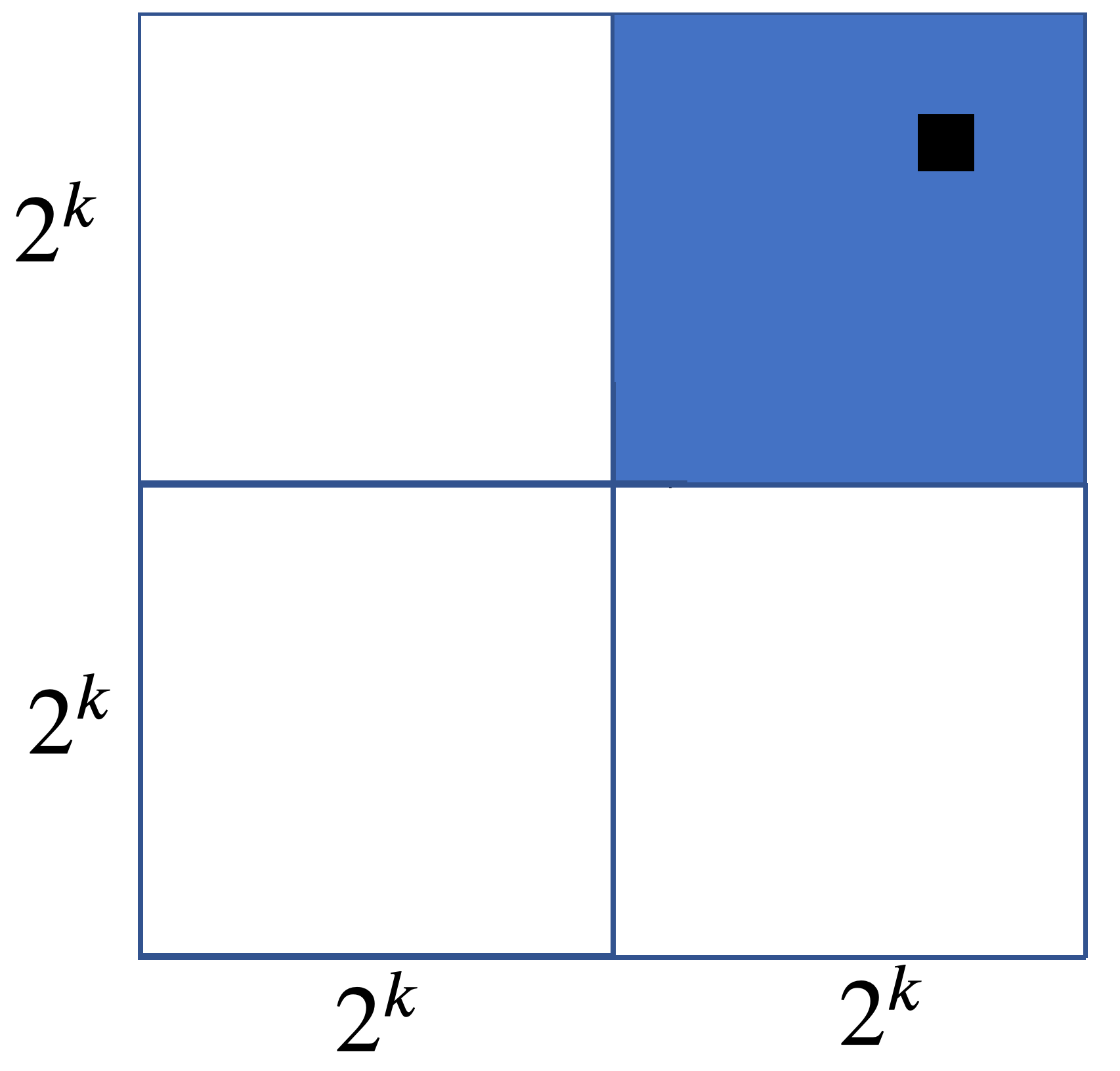
Inductive case. Assume that for $k \in \mathbb N$, the $2^k \times 2^k$ with one square removed can be tiled by triominoes. Now, consider an arbitrary grid of size $2^{k+1} \times 2^{k+1}$ with one square removed.
We split the grid into four $2^k \times 2^k$ grids. The square that is removed from our grid falls into one of these four subgrids. By our inductive hypothesis, each of these four grids can be tiled with triominoes with one square removed. So we have a tiling for the subgrid with our designated square removed and three other subgrids.
Our inductive hypothesis also implies we can tile the remaining three grids when their interior corners are removed:
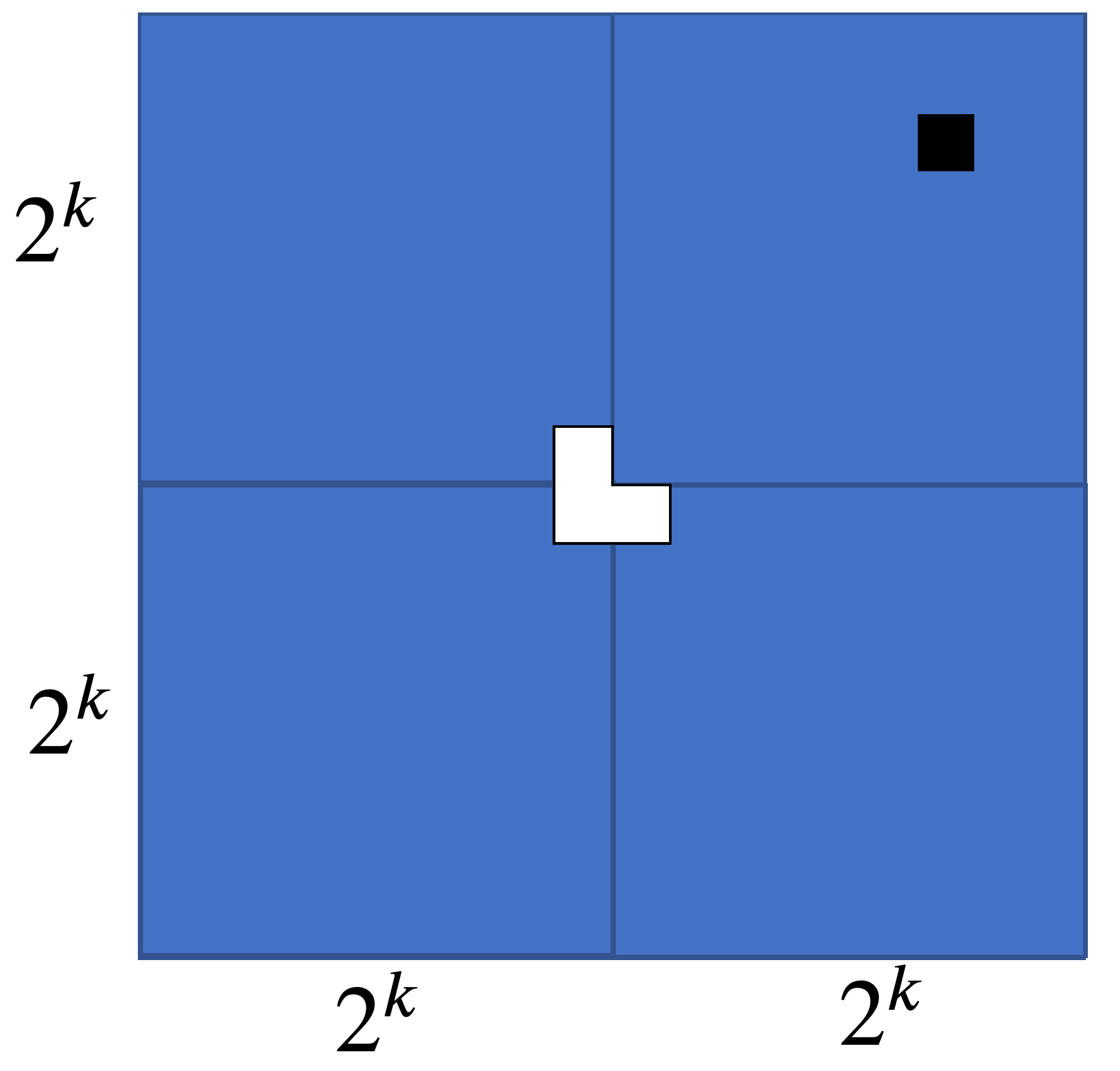
This leaves a spot for our last triomino, allowing us to tile the recomposed $2^{k+1} \times 2^{k+1}$ grid with only our designated tile missing. $\tag*{$\Box$}$
One thing that we haven't emphasized in this class is that induction can be applied to anything that is inductively defined, not just number. For instance, consider the following definition of a binary tree:
Example. A binary tree is either
Proof. We will show this by induction on the tree.
Base Case: A leaf. Every leaf's value is simply the number $m$ it contains, which is equal to $2^0 m$.
Inductive Case: Consider a node $n$. Assume for both of its subtrees $n_1$ and $n_2$, if their subtrees have the same value then they have the value $2^k m$ for some leaf value $m$.
Now assume all of $n$'s subtrees have the same value. Then the value of $n_1 = 2^k m$ for some $k$ and leaf value $m$. Since $n$'s subtrees have the same value, $n_2 = 2^k m$ as well. Then the value of $n = 2^k m + 2^k m = 2^{k+1} m$. $\tag*{$\Box$}$
"Theorem". All horses are the same color.
This is obviously false, so the following proof must be wrong. Try to spot the error.
Proof. We will that for all sets $H$ of horses, the horses in $H$ are all the same color. We do this by induction on $n = |H|$, the number of horses under consideration.
Base case. If $|H|=1$, then there is only one horse. A single horse is the same color as itself, so we are done.
Inductive case. Assume that any set of $n$ horses is the same color. Let $H$ be a set of $n+1$ horses, and consider two distinct horses in $H$. By the inductive assumption, if we remove either horse, then the remaining $n$ horses will be the same color. Thus, the first horse is the same color as the other horses, and similarly so is the second horse. Therefore all horses are the same color, completing the inductive proof. $\tag*{$\Box$}$
Can you spot the error?
The last technique we covered was the counting proof. If we can show that two sides of equality are counting precisely the same thing, then those two terms must be identical. One neat example was Pascal's identity:
Pascal's Identity. For all natural numbers $n \gt k \gt 0$, $$\binom{n}{k} = \binom{n-1}{k-1} + \binom{n-1}{k}.$$
Proof.Let $A$ be a set of $n \geq 2$ elements. We want to count the number of subsets of $A$ of size $k$, which is $\binom{n}{k}$. Choose an element $a \in A$ and a subset $B \subseteq A$ of size $k$. Then either $a \in B$ or $a \not \in B$; these two cases are disjoint. If $a \in B$, then $B$ contains $k-1$ elements in $A \setminus \{a\}$ and there are $\binom{n-1}{k-1}$ such sets. On the other hand, if $a \not \in B$, then $B$ contains $k$ elements in $A \setminus \{a\}$ and there are $\binom{n-1}{k}$ such sets. Together, this gives us $\binom{n-1}{k-1} + \binom{n-1}{k}$ subsets of $A$ of size $k$. $\tag*{$\Box$}$
That about covers it. These proof techniques should prove useful in Analysis of Algorithms and throughout your (hopefully extensive) mathematical studies.